Neural Networks for the Curious Mind
Published:
Neurons are the basic building block of modern Machine Learning. Over the past two decades, Machine Learning systems have achieved remarkable success across numerous disciplines and industries, making understanding its fundamentals no longer a matter reserved for experts, but a general skill and a precious opportunity for curious minds. The goal of this blog is to explain Neural Networks in a step-by-step manner that doesn’t require a strong math background.
Table of Contents
A Brief History of Neural Networks
The idea of neural networks goes back to the 1940s, when Warren McCulloch and Walter Pitts proposed a simple mathematical model of a neuron. In the 1950s and 1960s, researchers like Frank Rosenblatt developed the Perceptron, one of the first learning algorithms for single-layer networks.
Interest faded away in the 1970s, during the first ‘‘AI winter’’ 1, because early networks struggled with scaling to complex problems. Some big names in the field, as Marvin Minsky and Seymour Papert, turned their backs on the technique and even made specific efforts to discourage work on neural networks, claiming that its ability was limited to solving simple theoretical problems 2.
Things picked up again in the 1980s with the invention of backpropagation, an algorithm that allows neural networks to be trained efficiently. Then, A major breakthrough came in the 2010s, when advances in computing, big data, and new techniques led to the era of deep learning, making neural networks capable of remarkable feats, from image recognition to text generation. Today, neural networks are all around us, at the core of everything from recommendations on streaming platforms to self-driving cars.
Problem Formulation
Nowadays, a wide variety of tasks can be addressed with neural networks. To keep things straightforward and maintain our focus, this blog will concentrate on the classical supervised learning framework, aka, where the model learns to map inputs to known outputs in order to make predictions on new, unseen data. We’ll use this type of task as motivation for understanding why and how neural networks work.
Reminder in functions: Throughout this blog, the term function will appear frequently. Without going into detail, recall that a function is a mathematical rule that links each element from an input set to exactly one output.
Supervised learning stars from some labelled training dataset \(S\).
\[S=(x_i, y_i)_{i=1, \dots, N}\]As we just defined it, \(S\) is a set of samples \((x_i, y_i)\) composed by an input \(x_i\) and a label \(y_i\).
We assume that there is a function (unknown for us) \(f(\cdot)\), that outputs a label for each input :
\[y_i = f(x_i) + \nu,\]\(\nu\) is some small noise from the sampling process, that we can ignore for now.
Our objective is to learn a model \(\hat{f}(\cdot)\) of \(f(\cdot)\) 3.
What is a Neuron?
Understanding how a neuron works is an unavoidable step in grasping neural networks operation. For this purpose, let’s examine a basic artificial neuron alongside its biological inspiration.
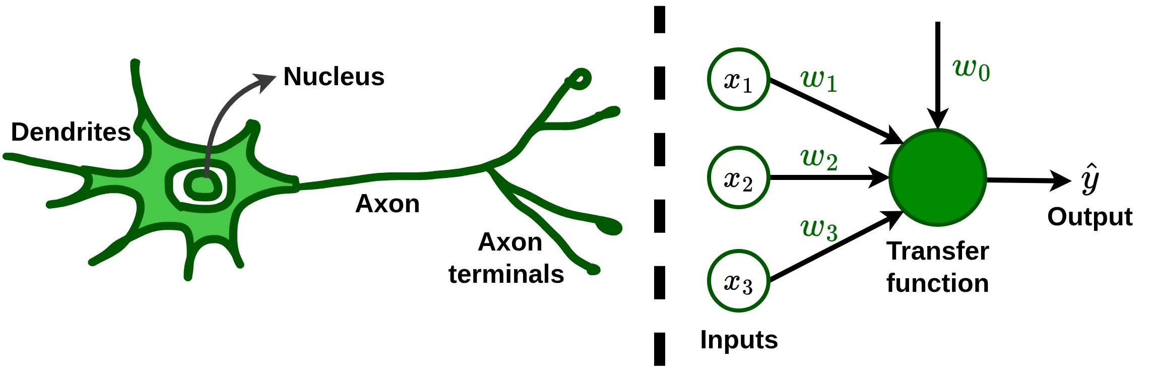
\(\{w_0, w_1, w_2, w_3\}\) are the parameters of the neuron, recall that a parameter is a special type of mathematical variable that influences the output or behavior of a mathematical object. We call weights \(\{w_1, w_2, w_3\}\) the parameters that scale the inputs, and bias \(w_0\) the independent parameter. The transfer function, is an arbitrary function used to combine the inputs, it’s tipically a linear combination.
To figure out how a neuron can help us solve problems, let’s jump right into a practical example.
An artificial neuron in action
Imagine that you are a farmer who wants to value his tractor in order to put it up for sale. You have the intuition that tractor prices depend in some way on \(x_1\), the engine size in \(\text{cm}^3\); \(x_2\), the number of kilometers driven; and \(x_3\), the number of hectares it can till per hour. This means assuming the existence of a \(f(x_1, x_2, x_3)\) that give us the price of a tractor, \(y\).
To model this, the most natural approach is to try a simple linear combination of the inputs, we can use a neuron where the transfer function is a standard linear regression. Notice that I add \(x_0 = 1\) to make bias compatible with the summation, this is just a notation precision.
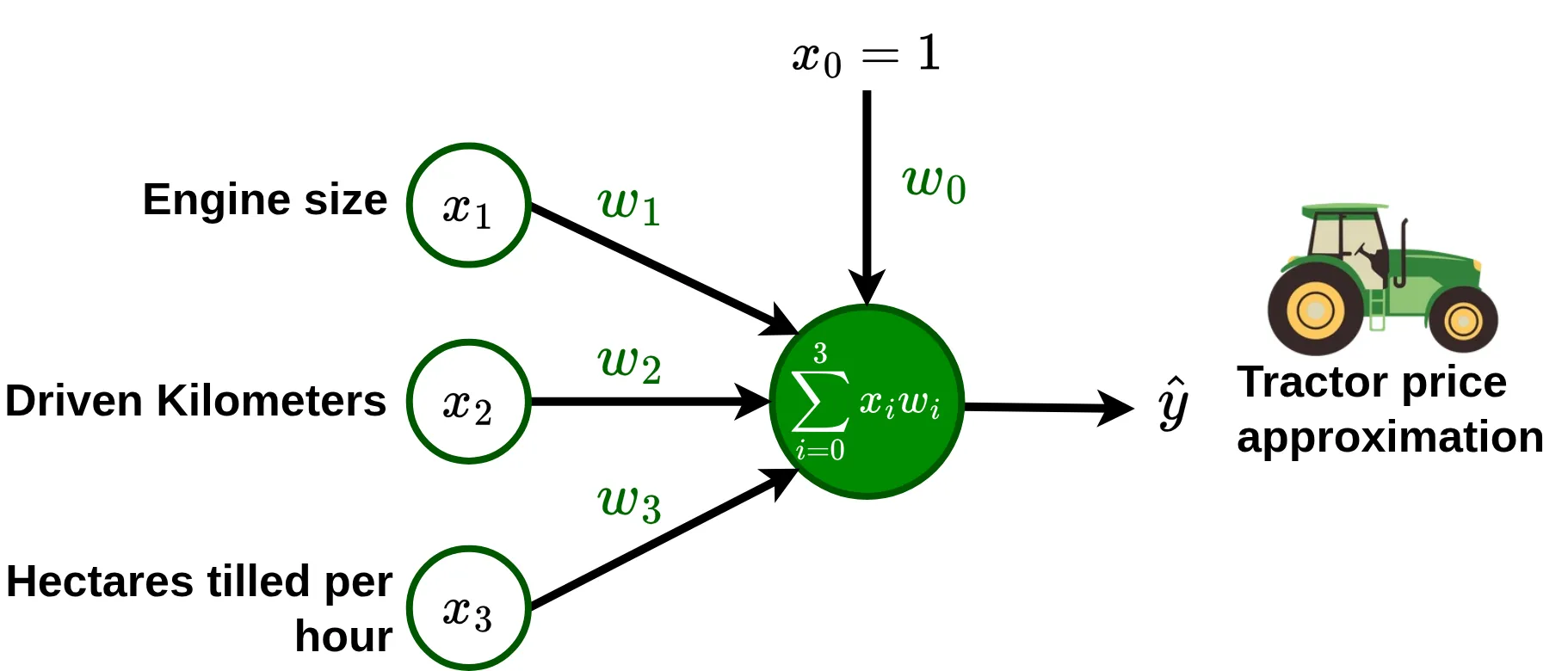
Thus, we can write the equation of the neuron that establishes the relationship between the inputs and the price of a tractor, as follows:
\[\hat{y} = \sum_{i=0}^{3}{x_iw_i} = (1)w_0 + x_1 w_1 + x_2 w_2 + x_3 w_3\]Next step is to assign appropriate values to our parameters. To do this, you take advantage of the annual farmers’ meeting in the region and ask some colleagues who sold their tractors in the last year about the features and sale price of their machines. With this information, you build a set of samples \(S\):
| \(x_1\) | \(x_2\) | \(x_3\) | \(y\) |
|---|---|---|---|
| 3 500 | 80 000 | 5 | 280 000 |
| 4 200 | 50 000 | 6 | 302 000 |
| 6 000 | 150 000 | 12 | 340 000 |
| 4 500 | 250 000 | 7 | 282 500 |
| 6 500 | 70 500 | 15 | 365 000 |
Under the supervised learning framework, we assume that a good model \(\hat{f}(x_1, x_2, x_3)\), will not only be capable of reproducing \(S\), but also of doing good prediction of tractor prices when using new input data.
The process of find the values \({w_0, w_1, w_2, w_3}\) that allow us to predict the prices \(y\) over \(S\), is called training. There are several algorithms that can be used to train a neuron, but, as they are out of the scope of this blog, we’re going to use simple trial and error. To assess how good a set of values is, we need a measure of the deviation between the real prices and the prices predicted by the neuron. This mesure is called loss. In this case, we’ll use the mean absolute error (MAE), that is just the mean of the distances (always positive) between the actual and predicted prices :
\[\text{MAE} = \frac{1}{n}\sum_{i=1}^{n} \lvert y_i-\hat{y_i} \rvert, \quad \text{where } n \text{ is the number of samples}\]Let’s do some iterations of the simple following process:
- Choice random values for the parameters.
- Compute our neuron for each sample in \(S\).
- Calculate the loss value.
- Stop the process when the loss is small enough, a MAE of less than 1000$ will be fine to us.
| Iteration | \(w_0\) | \(w_1\) | \(w_2\) | \(w_3\) | MAE |
|---|---|---|---|---|---|
| 1 | 10 000 | 1 500 | -50 | 1 000 | 351 300 |
| 2 | 130 000 | 30 | -0.2 | 5 000 | 23 080 |
| 3 | 250 000 | 15 | -0.2 | 2 100 | 7 160 |
| 4 | 200 000 | 24 | -0.1 | 1 100 | 2 550 |
| 5 | 200 000 | 25 | -0.15 | 1 000 | 985 |
After 5 iterations we found that best parameters are \(w_0 = 200 000, w_1 = 25, w_2= -0.15, w_3= 1 000\). Now, assuming that the collected samples are representative of actual market dynamics, you can estimate the price of your tractor, or virtually, the price of any other tractor under market conditions in your region over the last year, as that is the scope of the samples.
\[\begin{aligned} \hat{y} & = w_0 + x_1 w_1 + x_2 w_2 + x_3 w_3\\ \hat{y} & = 200 000 + (5 000 \cdot 25) + (10 000 \cdot -0.15) + (10 \cdot 1 000)\\ \hat{y} & = 200 000 + 125 000 - 1500 + 10 000\\ \hat{y} & = 336 500 \end{aligned}\]This way, your tractor, equipped with a 5 000 \(\text{cm}^3\) engine, 100 000 kilometers traveled and a capacity to till 10 hectares of land per hour, has an approximate retail price of 336 500$.
Note that the hypothesis that the collected samples represents well the actual process is a strong hypothesis; in real problems, a large number of good quality samples are required to ensure that the underlying function \(f(\cdot)\) is well represented.
Activation Functions for Introducing Non-linearity
Notice that our model for tractor prices prediction works because data fits our linear hypothesis well enough. Not all problems are this kind, in fact, most real-world problems we aim to solve with neural networks are highly complex and predominantly non-linear.
Since the neuron model is very convenient due to its flexibility and simplicity, we would like to bypass the linearity limitation by just adding an additional component.
Adding an activation function allows us to maintain the linear combination computation we studied earlier. The only additional step we need to take is to pass the result of our linear combination through this new, non-linear function. From now, I will use the notation \(g(z)\) to indicate an activation function that takes as input the output \(z\) of the linear transfer function.
There are many activation functions out there, and researchers and engineers are always introducing new ones. For now, I’ll focus on four of the simplest and most commonly used. Don’t worry if you’re not familiar with them, just remember that they are easy to compute and non-linear.
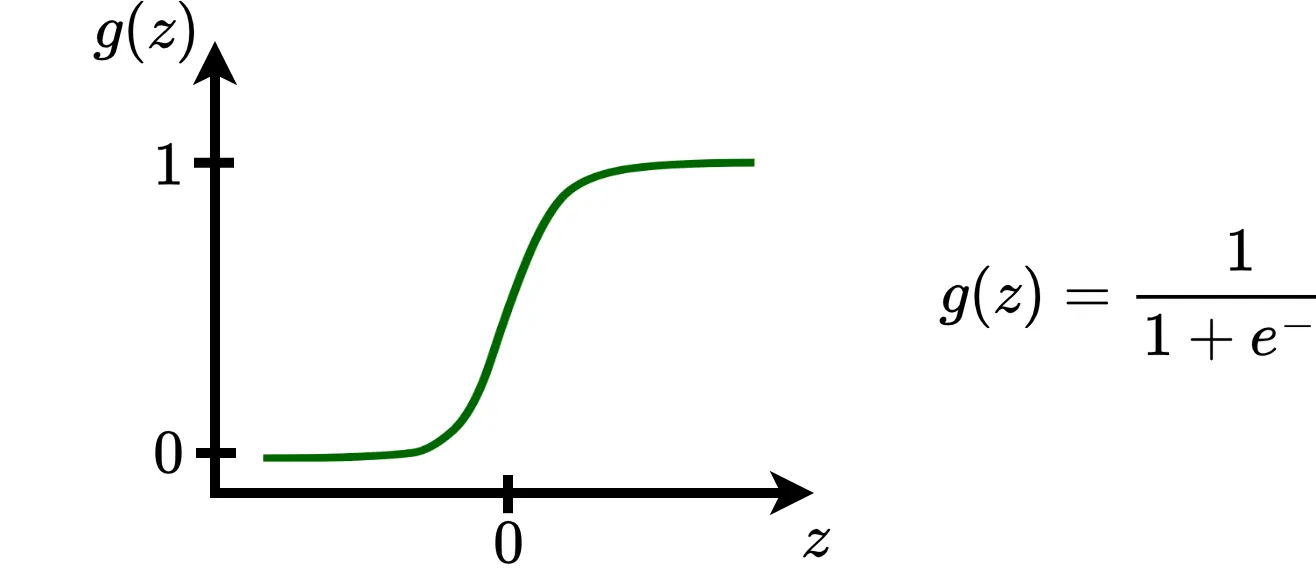
Sigmoid function is caracterized by its “S” shape. It’s output ranges between \(0\) and \(1\), which has proven useful for certain tasks, such as binary classification.
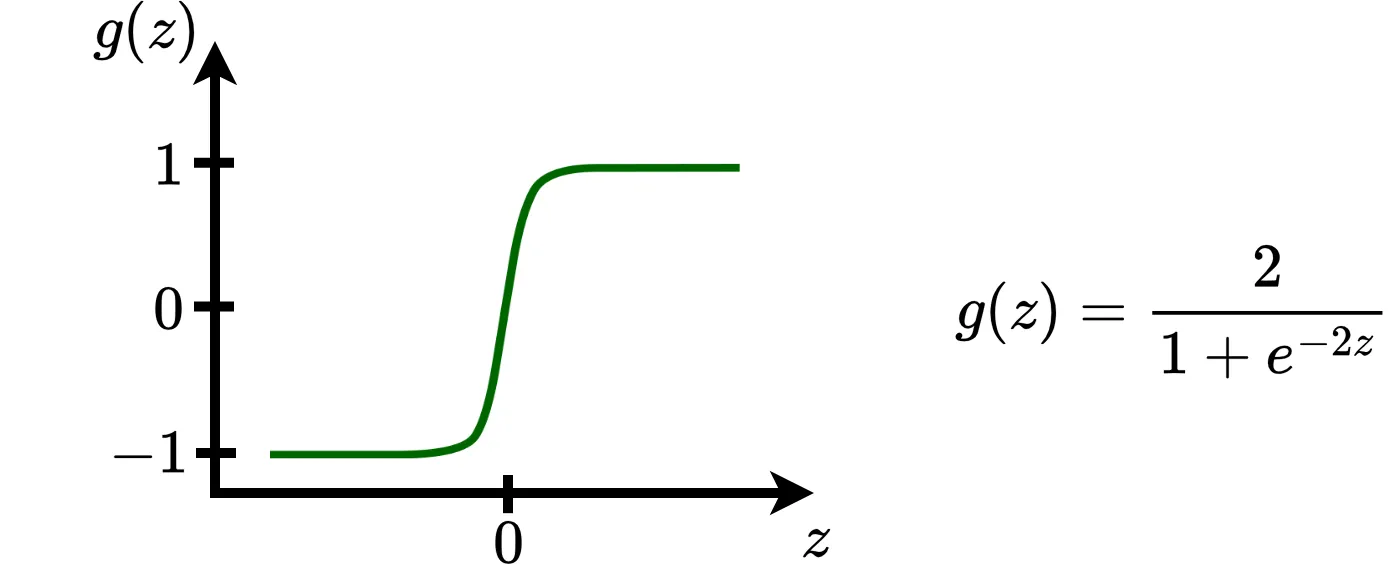
Tanh (hyperbolic tangent function) is a shifted version of the sigmoid. It’s output ranges between \(-1\) and \(1\).
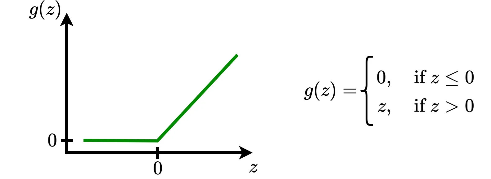
ReLU is the default choice in many neural networks. It is especially appreciated for its sparsity (it returns \(0\) for any input value \(\le 0\)), which helps to simplify the computational process.
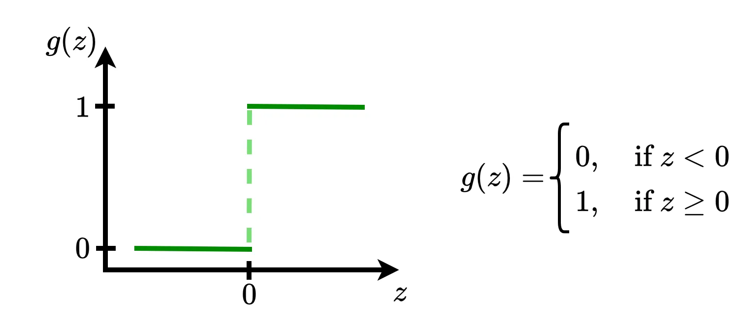
Binary step is a simple activation function based in a treshold principle. This function simply decides whether the neuron’s computation generates a signal or not. As you can see, it works like a switch, turning the output on or off depending on whether the input value is positive or negative.
Now, let’s see how activation functions allow neurons to represent much more complex and interesting functions, such as Boolean logic functions, which are at the heart of computing.
A non-linear neuron
Notice that in this toy example we know all the possible input-output \((x_i, y_i)\) pairs, in real life problems, we typically have access to only a subset of the samples.
The OR function between two elements is defined as follows:
| \(x_1\) | \(x_2\) | OR |
|---|---|---|
| 0 | 0 | 0 |
| 0 | 1 | 1 |
| 1 | 0 | 1 |
| 1 | 1 | 1 |
The analytic form of the OR function is :
Notice that it is non-linear, because the term where \(x_1 \text{ multiplies } x_2\) is of degree 2. Linear functions, when written as polynomials, only have terms of degree \(1\) or \(0\).
Despite this, we can still model the OR with a simple neuron .
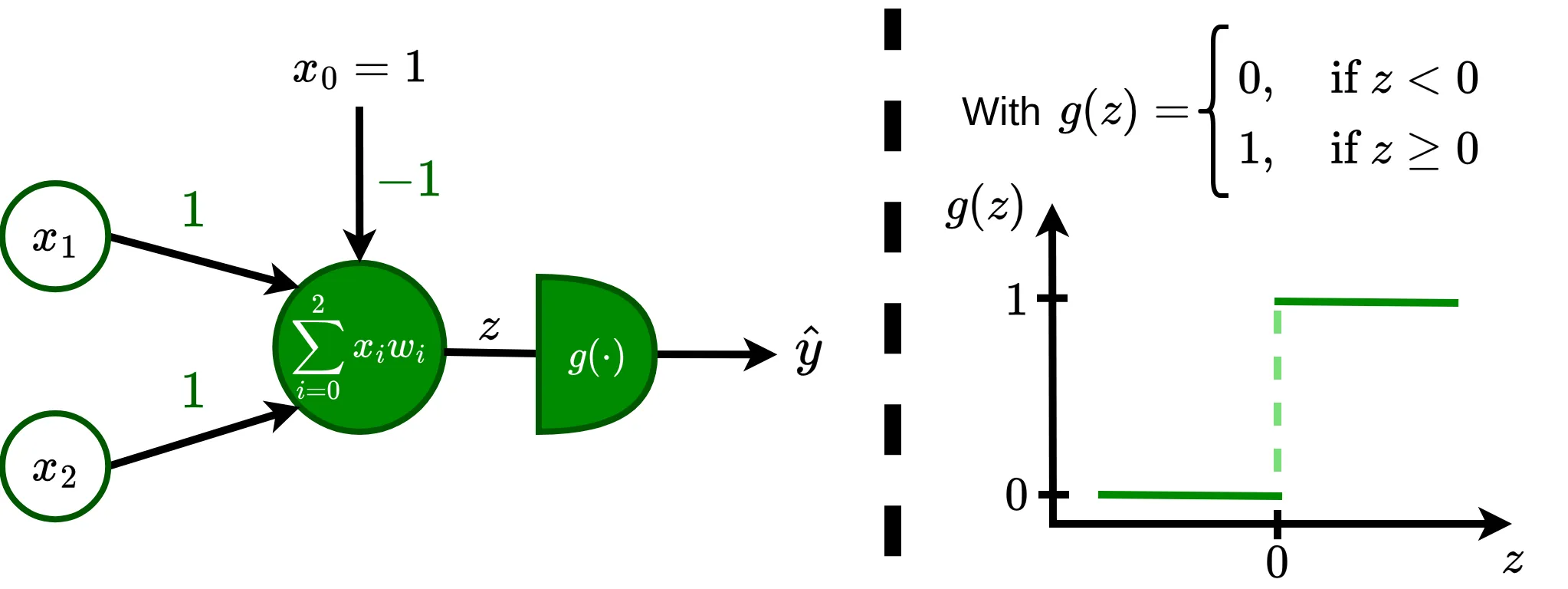
What’s fascinating is that even though the OR function is inherently non-linear, a single neuron equipped with a simple activation function can still capture this behavior, showing how a simple addition to the linear transfer function unlocks more complex modeling capacities.
The equation of a non-linear neuron is pretty similar to the one of the linear one, the only difference is an additional step, where we pass the result of the linear combination through an activation function.
\[\hat{y} = g(w_0 + x_1 w_1 + x_2 w_2), \quad \text{whith} \quad g(z) = \begin{cases} 0, &~ \text{if}~z \lt 0\\ z, &~ \text{if}~z \ge 0 \end{cases}\]Reminder on the degrees of a polynomial: The degree of a term is the sum of the exponents of the variables that appear in it and the degree of a polynomial is the highest degree of the polynomial’s terms. For example :
- The polynomial \(2x + 3\) has a degree \(1\), the term \(2x\) being of degree \(1\) and the term \(3\) of degree \(0\).
- The polynomial \(2xy + 3x^2 + 10\) has a degree \(2\), the term \(2xy\) being of degree \(2\), the term \(3x^2\) of degree \(2\) and the term \(10\) of degree \(0\).
What is a Neural Network?
A neural network is a parametric, learnable and biological inspired mathematical model. It is basically composed of neurons and connections between them. In this blog, we’ve used neurons to solve supervised learning problems, keep in mind, however, that neural networks are highly flexible and can be used to approximate virtually any function.
- They are parametric, meaning their behavior is determined by a set of parameters. The straight line \(y = \mathbf{m}x + \mathbf{b}\) is the most famous parametric model in the world, it has 2 parameters : \(\mathbf{m}\) (the slope) and \(\mathbf{b}\) (the intercept).
- They are learnable, which means we can automatically adjust these parameters, so the network gets better at mapping inputs to outputs.
- They are biological inspired because their design is loosely based on how the human brain works. Furthermore, they are made up of simple units, which pass information to each other. This idea comes from how real neurons communicate.
Neural Networks have 3 basic components:
- Neurons - that they take inputs, compute a transfer function, apply an activation function, and produce an output signal.
- Connections - that connect neurons to other neurons.
- Activation functions - a special kind of functions that introduce non-linearity.
Earlier in this blog, we realized the potential of a single neuron. Together, neurons become sophisticated non-linear function approximators whose abilities, as stunning as face recognition or image generation, emerge from the collaboration of many simple units.
Let’s use the same small neuron that I introduce in figure 1 to build one of the most widespread neural architectures: a feed forward neural network or fully connected neural network. As its name suggests, in this type of neural network, each neuron is connected to all neurons in the next layer.
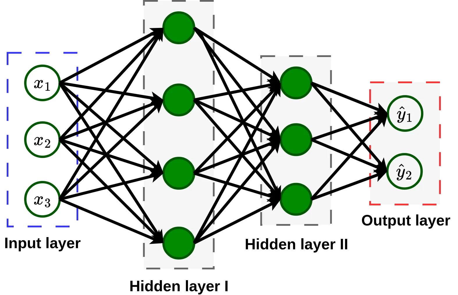
As you see, neural networks are organized in layers, which are essentially groups of neurons that work together to process an input and pass the output trought the connections to the next layer. The inputs themselves are considered the input layer, the final predictions form the output layer, and all intermediate layers, where the network learns to extract and combine meaningful information, are known as hidden layers.
When a neural network has one or more hidden layers, we describe it as deep. This is where the name deep learning comes from, referring to the use of “deep” neural networks.
Please note that although activation functions are applied to the output of each neuron, I include them as a component of the network, because we usually specify one activation function per layer.
What’s next ?
In this blog, we’ve learned what neural networks are and explore its main characteristics. But, to be honest, this is only half the story, The next step is learning how to make a neural network actually fit the data.
This is when training algorithms come in, they are methods in charge of the learning part: adjust the network’s parameters so it can make accurate predictions. I hope to write another post in the same lighthearted tone about training algorithms for neural networks. For now, I recommend this excellent blog by Christopher Olah on backpropagation (Disclaimer: this blog uses more technical terminology and requires a little more math, but it is extremely clear and comprehensive, moreover, Christopher is an extraordinary writer and scientist.)
For more in IA winters, there is a comprehensive Wikipedia article on the topic. ↩
For some good scientific drama and more historical context of this period, I highly recommend this super essay by Yuxi Liu. ↩
In Machine Learning, the notation \(\hat{\cdot}\) usually means approximation. ↩